Secondary plot (kinetics)

In enzyme kinetics, a secondary plot uses the intercept or slope from several Lineweaver-Burk plots to find additional kinetic constants.

For example, when a set of v by [S] curves from an enzyme with a ping–pong mechanism (varying substrate A, fixed substrate B) are plotted in a Lineweaver–Burk plot, a set of parallel lines will be produced.

The following Michaelis–Menten equation relates the initial reaction rate v₀ to the substrate concentrations [A] and [B]:

\begin{align} \frac{1}{v_0} &= \frac{ K_M^A}{v_\max {[}A{]}}+\frac{ K_M^B}{v_\max {[}B{]}}+\frac{1}{v_\max} \end{align}

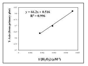
The y-intercept of this equation is equal to the following:

\begin{align} \mbox{y-intercept} = \frac{ K_M^B}{v_\max {[}B{]}}+\frac{1}{v_\max} \end{align}

The y-intercept is determined at several different fixed concentrations of substrate B (and varying substrate A). The y-intercept values are then plotted versus 1/[B] to determine the Michaelis constant for substrate B, $K_M^B$ , as shown in the Figure to the right. The slope is equal to $K_M^B$ divided by $v_\max$ and the intercept is equal to 1 over $v_\max$ .

Secondary Plot of enzyme system Horseradish Peroxidase and o-Phenylenediamine (with hydrogen peroxide as the second substrate)

Secondary Plot in Inhibition Studies

A secondary plot may also be used to find a specific inhbition constant, k_I.

For a competitive enzyme inhibitor, the apparent Michaelis constant is equal to the following:

\begin{align} \mbox{apparent } K_m=K_m\times \left(1+\frac{[I]}{K_I}\right) \end{align}

The slope of the Lineweaver-Burk plot is therefore equal to:

\begin{align} \mbox{slope} =\frac{K_m}{v_\max}\times \left(1+\frac{[I]}{K_I}\right) \end{align}

If one creates a secondary plot consisting of the slope values from several Lineweaver-Burk plots of varying inhibitor concentration [I], the competitive inhbition constant may be found. The slope of the secondary plot divided by the intercept is equal to 1/k_I. This method allows one to find the k_I constant, even when the Michaelis constant and v_max values are not known.

References

A. Cornish-Bowden. Fundamentals of Enzyme kinetics, Rev. ed., Portland: London, England, (1995) pp. 30-37, 56-57.
The Horseradish Peroxidase/ o-Phenylenediamine (HRP/OPD) System Exhibits a Two-Step Mechanism. M. K. Tiama and T. M. Hamilton, Journal of Undergraduate Chemistry Research, 4, 1 (2005).
J. N. Rodriguez-Lopez, M. A. Gilabert, J. Tudela, R. N. F. Thorneley, and F. Garcia-Canovas. Biochemistry, 2000, 39, 13201-13209.

This article is issued from Wikipedia - version of the 3/26/2013. The text is available under the Creative Commons Attribution/Share Alike but additional terms may apply for the media files.