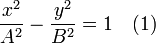
Lambert's problem

In celestial mechanics Lambert's problem is concerned with the determination of an orbit from two position vectors and the time of flight, solved by Johann Heinrich Lambert. It has important applications in the areas of rendezvous, targeting, guidance, and preliminary orbit determination.^[1] Suppose a body under the influence of a central gravitational force is observed to travel from point P₁ on its conic trajectory, to a point P₂ in a time T. The time of flight is related to other variables by Lambert’s theorem, which states:

The transfer time of a body moving between two points on a conic trajectory is a function only of the sum of the distances of the two points from the origin of the force, the linear distance between the points, and the semimajor axis of the conic.^[2]

Stated another way, Lambert's problem is the boundary value problem for the differential equation

\ddot {\bar r } = -\mu \cdot \frac {\hat r } {r^2}\ \

of the two-body problem for which the Kepler orbit is the general solution.

The precise formulation of Lambert's problem is as follows:

Two different times $\ t_1 \ ,\ t_2\$ and two position vectors $\bar r_1 = r_1 {\hat r}_1 ,\ \bar r_2 = r_2 {\hat r}_2\$ are given.

Find the solution $\bar r(t)$ satisfying the differential equation above for which

\bar r(t_1)=\bar r_1

\bar r(t_2)=\bar r_2.

Initial geometrical analysis

Figure 1:

F_1 \

: The centre of attraction

P_1 \

: The point corresponding to vector

\bar r_1\

P_2 \

: The point corresponding to vector

\bar r_2\

Figure 2: Hyperbola with the points

P_1 \

and

P_2 \

as foci passing through

F_1 \

Figure 3: Ellipse with the points

F_1 \

and

F_2 \

as foci passing through

P_1 \

and

P_2 \

The three points

$F_1 \$: The centre of attraction
$P_1 \$: The point corresponding to vector $\bar r_1\$
$P_2 \$: The point corresponding to vector $\bar r_2\$

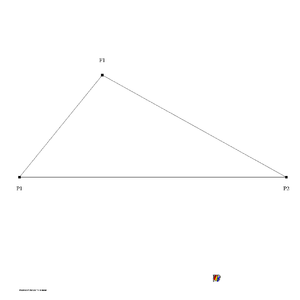
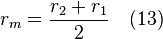
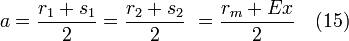
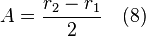
form a triangle in the plane defined by the vectors $\bar r_1\$ and $\bar r_2\$ as illustrated in figure 1. The distance between the points $P_1 \$ and $P_2 \$ is $2d \$ , the distance between the points $P_1 \$ and $F_1 \$ is $r_1 = r_m-A \$ and the distance between the points $P_2 \$ and $F_1 \$ is $r_2 = r_m+A \$ . The value $A \$ is positive or negative depending on which of the points $P_1 \$ and $P_2 \$ that is furthest away from the point $F_1 \$ . The geometrical problem to solve is to find all ellipses that go through the points $P_1 \$ and $P_2 \$ and have a focus at the point $F_1 \$

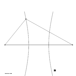
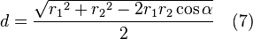
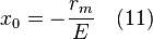
The points $F_1 \$ , $P_1 \$ and $P_2 \$ define a hyperbola going through the point $F_1 \$ with foci at the points $P_1 \$ and $P_2 \$ . The point $F_1 \$ is either on the left or on the right branch of the hyperbola depending on the sign of $A \$ . The semi-major axis of this hyperbola is $|A| \$ and the eccentricity $E\$ is $\frac{d}{|A|}\$ . This hyperbola is illustrated in figure 2.

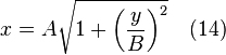
Relative the usual canonical coordinate system defined by the major and minor axis of the hyperbola its equation is

\frac{x^2}{A^2} - \frac{y^2}{B^2} = 1 \quad (1)

with

B = |A| \sqrt{E^2-1} = \sqrt{d^2-A^2} \quad (2)

For any point on the same branch of the hyperbola as $F_1 \$ the difference between the distances $r_2 \$ to point $P_2 \$ and $r_1 \$ to point $P_1 \$ is

$r_2 - r_1 = 2A \quad (3)$

For any point $F_2 \$ on the other branch of the hyperbola corresponding relation is

$s_1 - s_2 = 2A \quad (4)$

i.e.

r_1 + s_1 = r_2 + s_2 \quad (5)

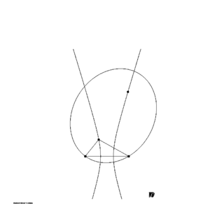
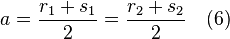
But this means that the points $P_1 \$ and $P_2 \$ both are on the ellipse having the focal points $F_1 \$ and $F_2 \$ and the semi-major axis

a = \frac{r_1 + s_1}{2} = \frac{r_2 + s_2}{2} \quad (6)

The ellipse corresponding to an arbitrary selected point $F_2 \$ is displayed in figure 3.

Solution of Lambert's problem assuming an elliptic transfer orbit

First one separates the cases of having the orbital pole in the direction $\bar r_1 \times \bar r_2\$ or in the direction $-\bar r_1 \times \bar r_2\$ . In the first case the transfer angle $\alpha$ for the first passage through $\bar r_2$ will be in the interval $\ 0 < \alpha < 180^\circ$ and in the second case it will be in the interval $180^\circ < \alpha < 360^\circ$ . Then $\bar r(t)$ will continue to pass through $\bar r_2$ every orbital revolution.

In case $\bar r_1 \times \bar r_2\$ is zero, i.e. $\bar r_1$ and $\bar r_2\$ have opposite directions, all orbital planes containing corresponding line are equally adequate and the transfer angle $\alpha$ for the first passage through $\bar r_2$ will be $180^\circ$ .

For any $\alpha$ with $\ 0 < \alpha < \infin$ the triangle formed by $P_1 \$ , $P_2 \$ and $F_1 \$ are as in figure 1 with

d = \frac{\sqrt{ {r_1}^2 + {r_2}^2 - 2 r_1 r_2 \cos \alpha}}{2} \quad (7)

and the semi-major axis (with sign!) of the hyperbola discussed above is

A = \frac{r_2 - r_1 }{2} \quad (8)

The eccentricity (with sign!) for the hyperbola is

E = \frac{d}{A} \quad (9)

and the semi-minor axis is

B = |A| \sqrt{E^2-1} = \sqrt{d^2-A^2} \quad (10)

The coordinates of the point $F_1 \$ relative the canonical coordinate system for the hyperbola are (note that $E$ has the sign of $r_2 - r_1$ )

x_0 = -\frac{r_m}{E} \quad (11)

y_0 = B \sqrt{{ \left(\frac{x_0}{A}\right) } ^2 - 1} \quad (12)

where

r_m = \frac{r_2 + r_1 }{2} \quad (13)

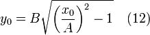
Using the y-coordinate of the point $F_2 \$ on the other branch of the hyperbola as free parameter the x-coordinate of $F_2 \$ is (note that $A$ has the sign of $r_2 - r_1$ )

x = A \sqrt{1+ {\left(\frac{y}{B}\right)}^2} \quad (14)

The semi-major axis of the ellipse passing through the points $P_1 \$ and $P_2 \$ having the foci $F_1 \$ and $F_2 \$ is

a = \frac{r_1 + s_1}{2} = \frac{r_2 + s_2}{2} \ = \frac{r_m + E x}{2} \quad (15)

The distance between the foci is

\sqrt{ {(x_0 - x)}^2 + {(y_0 - y)}^2} \quad (16)

and the eccentricity is consequently

e = \frac { \sqrt{{(x_0 - x)}^2 + {(y_0 - y)}^2}} {2 a} \quad (17)

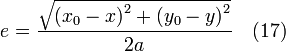
The true anomaly $\theta_1$ at point $P_1 \$ depends on the direction of motion, i.e. if $\sin \alpha$ is positive or negative. In both cases one has that

\cos \theta_1 = -\frac{(x_0+d) f_x + y_0 f_y}{r_1} \quad (18)

where

f_x = \frac{x_0 - x }{\sqrt{{(x_0 - x)}^2 + {(y_0 - y)}^2} } \quad (19)

f_y = \frac{y_0 - y }{\sqrt{{(x_0 - x)}^2 + {(y_0 - y)}^2} } \quad (20)

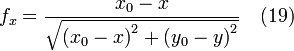
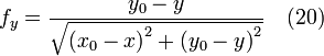
is the unit vector in the direction from $P_2$ to $P_1$ expressed in the canonical coordinates.

If $\sin \alpha$ is positive then

\sin \theta_1 = \frac{(x_0+d) f_y - y_0 f_x}{r_1} \quad (21)

If $\sin \alpha$ is negative then

\sin \theta_1 = -\frac{(x_0+d) f_y - y_0 f_x}{r_1} \quad (22)

With

semi-major axis
eccentricity
initial true anomaly

being known functions of the parameter y the time for the true anomaly to increase with the amount $\alpha$ is also a known function of y. If $t_2 -t_1$ is in the range that can be obtained with an elliptic Kepler orbit corresponding y value can then be found using an iterative algorithm.

In the special case that $r_1 = r_2$ (or very close) $A = 0$ and the hyperbola with two branches deteriorates into one single line orthogonal to the line between $P_1$ and $P_2$ with the equation

x = 0 \quad (1')

Equations (11) and (12) are then replaced with

x_0 = 0 \quad (11')

y_0 = \sqrt {{r_m}^2 - d^2} \quad (12')

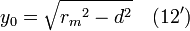
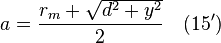
(14) is replaced by

x = 0 \quad (14')

and (15) is replaced by

a = \frac{r_m + \sqrt {d^2 + y^2}}{2} \quad (15')

Numerical example

Figure 4: The transfer time with : r₁ = 10000 km : r₂ = 16000 km : α = 120° as a function of y when y varies from −20000 km to 50000 km. The transfer time decreases from 20741 seconds with y = −20000 km to 2856 seconds with y = 50000 km. For any value between 2856 seconds and 20741 seconds the Lambert's problem can be solved using an y-value between −20000 km and 50000 km

Assume the following values for an Earth centred Kepler orbit

r₁ = 10000 km
r₂ = 16000 km
α = 100°

These are the numerical values that correspond to figures 1, 2, and 3.

Selecting the parameter y as 30000 km one gets a transfer time of 3072 seconds assuming the gravitational constant to be $\mu$ = 398603 km³/s². Corresponding orbital elements are

semi-major axis = 23001 km
eccentricity = 0.566613
true anomaly at time t₁ = −7.577°
true anomaly at time t₂ = 92.423°

This y-value corresponds to Figure 3.

With

r₁ = 10000 km
r₂ = 16000 km
α = 260°

one gets the same ellipse with the opposite direction of motion, i.e.

true anomaly at time t₁ = 7.577°
true anomaly at time t₂ = 267.577° = 360° − 92.423°

and a transfer time of 31645 seconds.

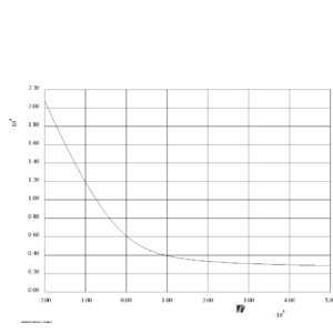
The radial and tangential velocity components can then be computed with the formulas (see the Kepler orbit article)

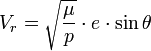
V_r = \sqrt{\frac {\mu}{p}} \cdot e \cdot \sin \theta \

V_t = \sqrt{\frac {\mu}{p}} \cdot (1 + e \cdot \cos \theta).

The transfer times from P₁ to P₂ for other values of y are displayed in Figure 4.

Practical applications

The most typical use of this algorithm to solve Lambert's problem is certainly for the design of interplanetary missions. A spacecraft traveling from the Earth to for example Mars can in first approximation be considered to follow a heliocentric elliptic Kepler orbit from the position of the Earth at the time of launch to the position of Mars at the time of arrival. By comparing the initial and the final velocity vector of this heliocentric Kepler orbit with corresponding velocity vectors for the Earth and Mars a quite good estimate of the required launch energy and of the maneuvres needed for the capture at Mars can be obtained. This approach is often used in conjunction with the patched conic approximation. This is also a method for orbit determination. If two positions of a spacecraft at different times are known with good precision from for example a GPS fix the complete orbit can be derived with this algorithm, i.e. an interpolation and an extrapolation of these two position fixes is obtained.

Open source code to solve Lambert's problem

From MATLAB central

PyKEP a Python library for space flight mechanics and astrodynamics (contains a Lambert's solver, implemented in C++ and exposed to python via boost python)

References

↑ E. R. Lancaster & R. C. Blanchard, A Unified Form of Lambert’s Theorem, Goddard Space Flight Center, 1968
↑ James F. Jordon, The Application of Lambert’s Theorem to the Solution of Interplanetary Transfer Problems, Jet Propulsion Laboratory, 1964

This article is issued from Wikipedia - version of the 5/1/2016. The text is available under the Creative Commons Attribution/Share Alike but additional terms may apply for the media files.